Initial Conditions for Field Fluctuations

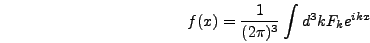
Although the field equations are solved in configuration space with each lattice point representing a position in space, the initial conditions are set in momentum space and then Fourier transformed to give the initial values of the fields and their derivatives at each grid point. As mentioned above, all of the expressions in this and the following two sections will be derived for a three dimensional lattice. Section 6.3.5 will explain how the results are altered in other dimensions. The Fourier transform $F_k$ in three dimensions is defined by

$$f(x) = {1 \over (2 \pi)^3} \int d^3k F_k e^{i k x}$$ (6.50)

It is assumed that no significant particle production has occurred before the beginning of the program, so quantum vacuum fluctuations are used for setting the initial values of the modes. The probability distribution for the ground state of a real scalar field in a FRW universe is given by [1,2]

$$P(F_k) \propto exp(-2 a^2 \omega_k \vert F_k\vert^2)$$ (6.51)

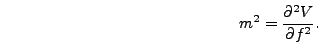
where

$$\omega_k^2 = k^2 + a^2 m^2,$$ (6.52)

$$m^2 = {\partial^2 V \over \partial f^2}.$$ (6.53)

Although $f$ is a real field the Fourier transform is of course complex, so this probability distribution is over the complex plane. The phase of $F_k$ is uniformly randomly distributed and the magnitude is distributed according to the Rayleigh distribution

$$P(\vert F_k\vert) \propto \vert F_k\vert exp(-2 a^2 \omega_k \vert F_k\vert^2).$$ (6.54)

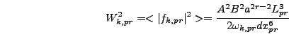
Note that this distribution gives the mean-squared value

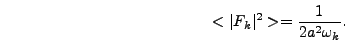$$<\vert F_k\vert^2> = {1 \over 2 a^2 \omega_k}.$$ (6.55)

To derive the expressions used for setting field values on the lattice we must modify equation (6.54) to account for a finite, discrete space, then account for the rescalings of field and spacetime variables, and finally discuss how to implement the Rayleigh distribution. In the rest of this section we do each of these in turn.

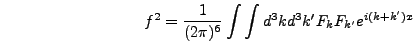
There are two steps involved in normalizing these modes on a finite, discrete lattice. First this definition has to be adjusted to account for the finite size of the box. This is necessary in order to keep the field values in position space independent of the box size. To see this consider the spatial average $<f^2>$.

$$f^2 = {1 \over (2 \pi)^6} \int \int d^3k d^3k' F_k F_{k'} e^{i (k + k') x}$$ (6.56)

$$<f^2> = {1 \over L^3 (2 \pi)^6} \int \int \int d^3x d^3k d^3... ...'} e^{i (k + k') x} = {1 \over L^3} \int d^3k \vert F_k\vert^2$$ (6.57)

where $L^3$ is the volume of the region of integration. So in order to keep $<f^2>$ constant as $L$ is changed the modes $F_k$ must scale as $L^{3/2}$.

Accounting for the discretization of the lattice is even easier. From the definition of a discrete Fourier transform (denoted here as $f_k$) in three dimensions

$$f_k \equiv {1 \over dx^3} F_k.$$ (6.58)

Note that values such as $<f^2>$ will be affected by changes in the lattice spacing, but this is reasonable since this spacing determines the ultraviolet cutoff of the theory. Without such a cutoff $<f^2>$ would be divergent.

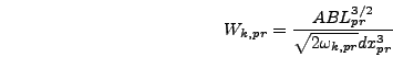
Putting these effects together gives us the following expression for the rms magnitudes, which we denote by $W_k$.

$$W_k \equiv \sqrt{<\vert f_k\vert^2>} = \sqrt{L^3 \over 2 a^2 \omega_k dx^6}$$ (6.59)

At a point $(i_1,i_2,i_3)$ on the Fourier transformed lattice the value of $k$ is given by

$$\vert k \vert = {2 \pi \over L} \sqrt{i_1^2 + i_2^2 + i_3^2}.$$ (6.60)

Next we rescale to program variables. The $L$, $dx$, and $k$ rescalings are determined by the rescaling of $x$ in equation (6.2), i.e.

$$L_{pr} = B L;\;dx_{pr} = B dx;\;k_{pr} = {k \over B}.$$ (6.61)

We can define a rescaling $\omega_{k,pr} \equiv \sqrt{k_{pr}^2 + m_{pr}^2} = \omega_k/B$ where $m_{pr} \equiv {a m \over B}$. (The extra factor of $a$ appears because the bare values $k$ and $m$ are measured in conformal and physical units respectively.) Then, taking into account the field rescaling $f_{pr} = A a^r f$

$$W_{k,pr}^2 = <\vert f_{k,pr}\vert^2> = {A^2 B^2 a^{2r-2} L_{pr}^3 \over 2 \omega_{k,pr} dx_{pr}^6}$$ (6.62)

Meanwhile the rescaled mass is given by

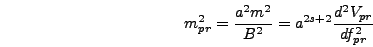$$m_{pr}^2 = {a^2 m^2 \over B^2} = a^{2s+2} {d^2 V_{pr} \over d f_{pr}^2}$$ (6.63)

Finally it remains to implement the Rayleigh distribution

$$P(\vert f_{k,pr}\vert) \propto \vert f_{k,pr}\vert exp(- \vert f_{k,pr}\vert^2 / W_{k,pr}^2)$$ (6.64)

Normalizing this distribution gives

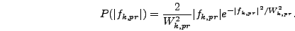$$P(\vert f_{k,pr}\vert) = {2 \over W_{k,pr}^2} \vert f_{k,pr}\vert e^{-\vert f_{k,pr}\vert^2/W_{k,pr}^2}.$$ (6.65)

To generate this distribution from a uniform deviate (i.e. a random number generated with uniform probability between $0$ and $1$) first integrate it and then take the inverse (see [3]), which gives

$$\vert f_{k,pr}\vert = \sqrt{- W_{k,pr}^2 ln(X)}$$ (6.66)

where $X$ is a uniform deviate.

There are two more points to note in setting the initial conditions for the fluctuations. The first is simply that the scale factor is set to $1$ at the beginning of the calculations and may thus be dropped from the equations. The second is that the phases of all modes are random and uncorrelated, so they are each set randomly. The expression for the field modes is thus

$$f_{k,pr} = e^{i \theta} \sqrt{- W_{k,pr}^2 ln(X)}$$ (6.67)

where

$$W_{k,pr} = {A B L_{pr}^{3/2} \over \sqrt{2 \omega_{k,pr}} dx_{pr}^3}$$ (6.68)

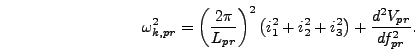
and $\theta$ is set randomly between $0$ and $2 \pi$. The frequency $\omega_{k,pr}$ for a given point $(i_1,i_2,i_3)$ on the momentum space lattice is given by

$$\omega_{k,pr}^2 = \left({2 \pi \over L_{pr}}\right)^2 \left(i_1^2 + i_2^2 + i_3^2\right) + {d^2 V_{pr} \over d f_{pr}^2}.$$ (6.69)