We should note that there are many important topics in quantum mechanics that we will not touch in this paper, including angular momentum, commutation relations, bra-ket notation, and more. What we are going to discuss is how to use and interpret wavefunctions. Moreover, the way we are going to present the postulates of quantum mechanics is not the most generalizable, but it is in our opinion the simplest form for understanding and solving basic problems.
For a classical system made up of particles, you can completely specify the state of the system by giving the position and momentum (or equivalently velocity) of every particle in the system at any particular time. If you consider one particle whose position and momentum is known at this initial time, then if you know all the forces acting on that particle you can write down equations which tell you exactly what its position and momentum will be at any future time. Note that instead of specifying the forces you can specify the potential energy function, which is equivalent: force is the gradient of potential.
In quantum mechanics the situation is a little more complicated. The systems that you study are still made of particles, and the basic procedure is in some ways similar: You measure the state of a particle at some initial time, you specify the forces acting on that particle (or equivalently, the potential energy function describing those forces), and quantum mechanics gives you a set of equations for predicting the results of measurements taken at any later time. There are two key differences between these two theories, however. First of all, the state of a particle in quantum mechanics is not just given by its position and momentum but by something called a "wavefunction." Secondly, knowing the state of a particle (ie its wavefunction) does not enable you to predict the results of measurements with certainty, but rather gives you a set of probabilities for the possible outcomes of any measurement.
The wavefunction which describes the state of a particle is often denoted by the letter Y (spelled "psi" and pronounced "sigh"). It is a complex function which is defined everywhere in space. (Click to jump to a brief description of complex numbers and magnitudes.) No matter what state your particle is in, its wavefunction has some complex value at every point in the universe.
A typical quantum mechanics problem would thus run as follows: You start with a particle in an unknown state subject to a known set of forces, such as an electron in an electromagnetic field. You perform a measurement on that particle that tells you its state, ie its wavefunction. You let it evolve for a certain amount of time and then take another measurement. Quantum mechanics can tell you what result to expect from this second measurement. There are thus three questions we need to address in formulating the basic theory of quantum mechanics.
In order to keep this topic as simple as possible, we're going to start by living in a very simple universe. Our universe has only three points: x=1, x=2, and x=3. Our particle must be on exactly one of those points. It cannot be anywhere else, including in between them. Since those three points define the whole universe, the wavefunction itself is defined at all three of those points, and nowhere else. So Y is just three complex numbers, which might look something like this.
Now, if we sum up the probabilities of all three locations, we get the odds that the particle will be in any one of those three states. Since we've already said that the particle must be at one of those states, we should get a probability of 1. But at the moment, we find a total probability of 18. That means this wavefunction is unnormalized: it can tell us the relative probabilities of two positions, but not the absolute probabilities of any of them. To normalize it, we multiply all the values by a constant, to make the total probability equal to 1. In this case, we have to multiply every value of |Y|2 by 1/18, which means we multiply every value of Y by the square root of 1/18. This will keep all the relative probabilities the same, but ensure that the total probability of finding the particle somewhere is 1.
So now, at our three places, we have the following.
Now, by applying some basic probability theory to those numbers, we can answer another very important question: if I had a lot of particles in exactly this state, and I measured all their positions, what would the average result be? This is called the "expectation value" of position and is often written as <x>. It is calculated as: one times (probability of x=1), plus two times (probability of x=2), plus three times (probability of x=3). (Click to jump to a brief description of expectation values and this calculation.) You should verify for yourself that this gives 42/18=7/3. So if we had a whole bunch of these particles and measured them all, and averaged all the positions, the average position would be at 2![]() ; even though, of course, none of the particles is actually at that position.
; even though, of course, none of the particles is actually at that position.
I want to make it clear what we've introduced so far. We've said that "the magnitude of the wavefunction squared gives the probability of finding the particle at a particular position." This is a totally out-of-the-air rule; or, to put it another way, a fundamental postulate of quantum mechanics, that we will not make any attempt to justify.
Based on that, we applied some basic probability math (no new Physics or crazy ideas) to do two things. First, we normalized Y so that the total probability sum was one. Second, we calculated the expectation value of position. Hopefully, there was nothing too surprising in any of that.
We're going now to repeat that whole exercise, but for a slightly more realistic case, where the particle can be anywhere on the x axis (instead of only in three possible places). Of course, the math will get a bit hairier, and our sums will become integrals, but all the basic ideas will be the same.
(Of course, we could make the universe even more complicated by making it three-dimensional, such as, say, the real world. But we'll stick entirely with one dimension in this paper. That means that the answers we find for position and momentum will be numbers, not vectors.)
As before, let's start by assuming we've already calculated Y. And just for fun, let's say it wound up looking like exactly one wavelength of a sin wave.
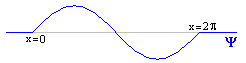
At any given point, Y has some value: for instance, Y(p/2)=1. By analogy to what we did before, you might suppose that the square magnitude of this value gives the probability of finding the particle there: so the probability (unnormalized) of finding the particle at x=p/2 is 1.
But that isn't quite true. x=p/2 is some teeny tiny little point, one of infinitely many such points in the range 0<x<2p. The probability of being at exactly that point, or any other specific position, is zero. So Y does not exactly give a probability but a "probability density," and our golden rule is: the integral of |Y|2 between any two points, gives the probability of the particle appearing between those two points. For instance, ![]() |Y|2dx gives the probability of finding the particle somewhere between x=0 and x=1.
|Y|2dx gives the probability of finding the particle somewhere between x=0 and x=1.
If you haven't worked with probability densities before, this idea takes a bit of getting used to, but if you play with it, it becomes very natural. You find that in areas where Y is uniformly zero, the probability is zero. In areas where Y is high, the probabilities tend to be high. You find that the probability of being at any exact point is zero (as we said earlier), since the integral from any number to itself is always zero. The probabilities sum in a natural way: the odds of being between 0 and 1, plus the odds of being between 1 and 2, give you the odds of being between 0 and 2. All this corresponds to what you would expect. (Of course, remember that we're working with |Y|2 and not just Y. So you never have a negative probability. In our example, the right half of the wave has exactly the same probability as the left half.)
And of course, we have a normalization condition, similar to the one we had in the discrete case. The integral
![]()
gives the probability of finding the particle anywhere, and should be 1.
Question: The wavefunction given in the example above is unnormalized. What do we have to do to it (what do we have to multiply it by) in order to normalize it? We highly recommend you try to figure this out for yourself before reading any further—these little exercises are an important way to make sure you're still following along, and haven't missed anything.
Answer: You have to multiply Y by 1/![]() . To confirm that answer, you have to calculate
. To confirm that answer, you have to calculate ![]() |Y|2dx for the original function given above. The result of this integral works out to be p. So once we divide Y by
|Y|2dx for the original function given above. The result of this integral works out to be p. So once we divide Y by ![]() then
then ![]() |Y|2dx will give us 1, which is what we want.
|Y|2dx will give us 1, which is what we want.
So we now have a properly normalized Y:
What about the expectation value? In our discrete-position universe, we calculated the expectation value by doing a sum: the x-value of a point, times the normalized probability of the particle appearing at that point, summed over all the points. As you might expect, we will calculate expectation value by the same basic principal, but using an integral: ![]() x|Y|2dx. If we had a million particles with this particular Y, and we measured all their positions and averaged the results, this formula would give us the average.
x|Y|2dx. If we had a million particles with this particular Y, and we measured all their positions and averaged the results, this formula would give us the average.
So, this is another good point for a do-it-yourself exercise. First, looking at the drawing of Y above, what would you intuitively think the expectation value of position for the particle would be? (In other words, on average, where would you expect to find the particle?) Now, actually do the integral. Did you get the result you expected?
We're done with position. So before we go on, let's once again summarize where we are.
We have essentially learned only one rule, which is that |Y|2 gives you the probability of finding a particle at a given position. But we've layered a considerable amount of math onto that rule.
But if you're on top of all the math, then we've just learned one little rule so far, which is all you need for position.
To answer this question, we're going to start with a special case that turns out to be quite simple. If a particle is in a state described by Y=e5ix/![]() then its momentum is 5. No ambiguity, no probabilities, the momentum is just 5. (Don't worry about the normalization of this wavefunction for the moment; we'll return to that point later.)
then its momentum is 5. No ambiguity, no probabilities, the momentum is just 5. (Don't worry about the normalization of this wavefunction for the moment; we'll return to that point later.)
Now, as you might guess, there is nothing particularly special about the number 5. If Y=e7ix/![]() then the momentum is 7. In general, if Y=eipx/
then the momentum is 7. In general, if Y=eipx/![]() for any constant p, then the momentum of the particle is exactly p.
for any constant p, then the momentum of the particle is exactly p.
Functions of this form (Y=eipx/![]() ) are known as the basis states of momentum, which means they represent particles that have exactly specified momentum. They may seem like such a special case that it isn't very interesting: how often is Y going to happen to be in just exactly that form? But in fact, the basis states are the key to the whole process. The general strategy is to represent Y as a sum of different basis states, and once Y is represented in that way, you can easily get all the information you need about momentum.
) are known as the basis states of momentum, which means they represent particles that have exactly specified momentum. They may seem like such a special case that it isn't very interesting: how often is Y going to happen to be in just exactly that form? But in fact, the basis states are the key to the whole process. The general strategy is to represent Y as a sum of different basis states, and once Y is represented in that way, you can easily get all the information you need about momentum.
We can illustrate the key "momentum strategy" by moving to a slightly more complicated example.
![]()
This is not a basis state, so the momentum is not exactly specified. But this wavefunction is a sum of two different basis states, e23ix/![]() and e42ix/
and e42ix/![]() . We can therefore say with confidence that the momentum of the particle must be either 23 or 42. To find the relative probabilities, we look at the coefficients—the numbers multiplied by these basis states—and we square them. (2)2=4, |2+2i|2=8, so the particle is twice as likely to have momentum 42 as it is to have momentum 23.
. We can therefore say with confidence that the momentum of the particle must be either 23 or 42. To find the relative probabilities, we look at the coefficients—the numbers multiplied by these basis states—and we square them. (2)2=4, |2+2i|2=8, so the particle is twice as likely to have momentum 42 as it is to have momentum 23.
In summary, there are two key rules you need to know about momentum.
![]()
where |f(3)|2 gives the relative probability of finding the particle with momentum 3; and, in general, |f(p)|2 gives the relative probability of finding the particle with momentum p, for any p. Since there are infinitely many possibilities, we aren't looking for a bunch of individual numbers: we're looking for one general function, f(p), that will give us all our coefficients and therefore all our probabilities.
Finally, moving (as we did with position) from a discrete world to a continuous world where p can be any real number, what we really want to write is:
![]()
The numerical coefficient in front of the integral is just a convention that makes certain equations simpler. Aside from that, this formula simply says "We are representing Y as a combination of different momentum basis states eipx/![]() , each with its own coefficient f(p)." Any function Y(x) can be written in this form, and once you do, you can find the probability of the particle being in any particular momentum range. Some of you may recognize this as the formula for a Fourier Transform. Click for a brief introduction to Fourier transforms, including how to invert this formula to find f(p) for a given wavefunction Y(x).
, each with its own coefficient f(p)." Any function Y(x) can be written in this form, and once you do, you can find the probability of the particle being in any particular momentum range. Some of you may recognize this as the formula for a Fourier Transform. Click for a brief introduction to Fourier transforms, including how to invert this formula to find f(p) for a given wavefunction Y(x).
Of course, moving from a discrete world to a continuous world forces us to view things a little differently, exactly as it did in the case of position. The squared magnitude |f(p)|2 does not represent the probability of finding the particle with momentum p exactly—that probability will always be zero. Instead, you integrate |f(p)|2 between any two numbers to find the probability of the momentum falling into that range: for instance, ![]() |f(p)|2 dp gives the probability that the particle will have a momentum between 0 and 1. Analogously to the position case,
|f(p)|2 dp gives the probability that the particle will have a momentum between 0 and 1. Analogously to the position case, ![]() p|f(p)|2 dp gives you the expectation value of p.
p|f(p)|2 dp gives you the expectation value of p.
Dealing with a continuous world allows us to finally address the question of normalization that we've been ducking so far in this section. A wavefunction with exact momentum such as Y=e5ix/![]() cannot be normalized. (Try it!) This means that you can't have a nonzero probability of having your momentum exactly equal to 5, just as the probability of the position being at exactly any point was zero. A wavefunction of the form
cannot be normalized. (Try it!) This means that you can't have a nonzero probability of having your momentum exactly equal to 5, just as the probability of the position being at exactly any point was zero. A wavefunction of the form
![]()
can be normalized, however. Recall that to normalize Y you set ![]() |Y(x)|2 dx=1, meaning the total probability of finding the particle somewhere is equal to one. It turns out that if you do that you will necessarily find that
|Y(x)|2 dx=1, meaning the total probability of finding the particle somewhere is equal to one. It turns out that if you do that you will necessarily find that ![]() |f(p)|2 dp=1, meaning that the total probability of finding the particle with some momentum is equal to one. This fact, which follows directly from the properties of Fourier Transforms, is one of those cases where the math seems to almost magically do what it has to in order to give you the right answer.
|f(p)|2 dp=1, meaning that the total probability of finding the particle with some momentum is equal to one. This fact, which follows directly from the properties of Fourier Transforms, is one of those cases where the math seems to almost magically do what it has to in order to give you the right answer.
Since the function f(p) contains all the information that Y(x) contains, but represented in a different form, the two functions Y(x) and f(p) are sometimes referred to as the "position representation" and the "momentum representation" of the wavefunction, respectively. This is pretty elegant because the way you treat f(p) to find momentum probabilities is exactly the way you treat Y(x) to get position probabilities.
So let's summarize what we've learned about momentum.
But the bad news is, we used one set of arbitrary looking rules for position, and a completely different set of arbitrary looking rules for momentum. The wavefunction is supposed to tell us everything we would ever want to know about a particle, including its kinetic energy, angular momentum, hair color, cup size, and comparable worth. Are we going to have to learn a whole new set of rules for each observable quantity?
The answer is no. In fact, there is one absolutely general rule that enables you to analyze a wavefunction to find the probabilities of any measurable quantity about a particle. Unfortunately, it's a pretty ugly looking sort of rule, which is why we've been putting it off. Now we're going to get there, and the way we're going to get there is by talking some more about momentum.
All of that applies to any other measurable quantity. So for instance, there are certain functions that represent basis states of energy. If the wavefunction is in a basis state of energy, then the energy is determined; if it isn't, you can rewrite it as a sum of different basis states of energy, and use their coefficients to find the probabilities of different energy values.
But different observables have different basis states. The function eipx/![]() happens to be a basis state for momentum, but it isn't a basis state for all quantities. In fact, the Heisenberg Uncertainty Principle guarantees that you can never be in a basis state for everything at once: if some things are precisely determined, other things are vague and probabilistic! (The rules we've given so far are actually enough to derive the Heisenberg Principle for position and momentum. Think about what we've said so far and try to convince yourself that a particle couldn't be in a state of exact momentum and position. Click for an intuitive derivation of the uncertainty principle.)
happens to be a basis state for momentum, but it isn't a basis state for all quantities. In fact, the Heisenberg Uncertainty Principle guarantees that you can never be in a basis state for everything at once: if some things are precisely determined, other things are vague and probabilistic! (The rules we've given so far are actually enough to derive the Heisenberg Principle for position and momentum. Think about what we've said so far and try to convince yourself that a particle couldn't be in a state of exact momentum and position. Click for an intuitive derivation of the uncertainty principle.)
What we need in order to generalize to all the different things we want to measure is to know their basis states. How do you find the basis state for a particular quantity? In order to answer that, we first have to introduce the mathematical concept of an operator. This is pretty simple, as concepts go: an operator is something you do to a function, and you get a different function. For instance, an operator might be "add seven" or "take the second derivative and then take the sin" or something like that.
In quantum mechanics, every measurable quantity is associated with an operator. For instance, the position operator happens to be "x" meaning "any function you give me, I will multiply by x." The momentum operator is "—i![]()
![]() " meaning "any function you throw at me, I will take the first derivative of it, and then multiply by —i
" meaning "any function you throw at me, I will take the first derivative of it, and then multiply by —i![]() ." So if you act with the position operator on the function x5 you get x6; if you act with the momentum operator on x5 you get —5i
." So if you act with the position operator on the function x5 you get x6; if you act with the momentum operator on x5 you get —5i![]() x4. Nothing too fancy-looking there, right? Doesn't look particularly useful, but at least it isn't hard.
x4. Nothing too fancy-looking there, right? Doesn't look particularly useful, but at least it isn't hard.
Now, what happens when you act on Y=e5ix/![]() with the momentum operator? (Try this yourself to make sure you get the same answer we do!) You get 5e5ix/
with the momentum operator? (Try this yourself to make sure you get the same answer we do!) You get 5e5ix/![]() . Note that you got back the exact same function you started with, times 5. It is exactly this fact that makes e5ix/
. Note that you got back the exact same function you started with, times 5. It is exactly this fact that makes e5ix/![]() a basis state with momentum 5: when you act on it with the momentum operator, you get the same function back, times 5.
a basis state with momentum 5: when you act on it with the momentum operator, you get the same function back, times 5.
This brings us to the general rule for finding basis states, and it's a really ugly and arbitrary-looking rule, but it is a key postulate of quantum mechanics, so it's worth stating on its own:
When the operator for a particular quantity, acting on a wavefunction, produces that same wavefunction times a constant, then that wavefunction is a basis state for that quantity, and the constant is the value for that quantity.
This is not only ugly, it's hard to say. We can't make it less ugly, but we can make it easier to say by introducing some terminology. Any function that has this property (the operator returns the same function times a constant) is called an eigenfunction of the operator, and the constant is called its eigenvalue. We can now state our general rule more succinctly:
The eigenfunctions of an operator represent its basis states, and their eigenvalues are the corresponding values of the measurable quantity.
We can get even more concise by writing it mathematically. Let "A" be an operator, so "AY" means "the operator A acting on Y." And let "a" be a constant. Then we can define "Y" as an eigenfunction (or basis state) of A and "a" as an eigenvalue, all by writing:
AY = aY (—>"A operating on Y produces a times Y")
Since this is so abstract, it's worth coming back to the simple example we started with, because the example really says it all. The momentum operator is —i![]()
![]() . It just so happens that if Y=ei5x/
. It just so happens that if Y=ei5x/![]() , then when you act on Y with the momentum operator you get 5Y. This tells us that Y=e5ix/
, then when you act on Y with the momentum operator you get 5Y. This tells us that Y=e5ix/![]() is a basis state (or eigenfunction) that represents a particle with a definite momentum of 5 (the eigenvalue).
is a basis state (or eigenfunction) that represents a particle with a definite momentum of 5 (the eigenvalue).
So—for those of you keeping track at home—here's what we've done so far. We have introduced two extremely arbitrary-looking and ugly postulates. One is "the basis states are the wavefunctions with the peculiar property that, when you operate on them, you get them back times a constant." The other is "the operator for momentum is —i![]()
![]() ". Using these two rules, we've been able to easily prove the rule that seemed totally arbitrary in the last section, "the basis states of momentum are of the form Y=eipx/
". Using these two rules, we've been able to easily prove the rule that seemed totally arbitrary in the last section, "the basis states of momentum are of the form Y=eipx/![]() ." We can now see that that formula wasn't arbitrary; it was a special case of a general principal. Still, this hardly seems like an improvement, does it?
." We can now see that that formula wasn't arbitrary; it was a special case of a general principal. Still, this hardly seems like an improvement, does it?
But the reason we went through all that is because, once we have generalized in this fashion, we can very easily get at all the other observable quantities. The reason is that virtually all observable quantities are built from position and momentum, and the way you build them in quantum mechanics is through the operators. (The main exception is spin.)
For instance, consider kinetic energy. Classically, we know that kinetic energy is p2/2m. (This is another way of writing the more familiar "½mv2.") In quantum mechanics, the same rule applies, except that instead of numbers we're working with operators. The momentum operator is —i![]()
![]() . We find kinetic energy by "squaring" that operator (ie doing it twice) and then dividing by 2m, so the kinetic energy operator is
. We find kinetic energy by "squaring" that operator (ie doing it twice) and then dividing by 2m, so the kinetic energy operator is ![]() . We can use this to find the basis states for kinetic energy, and all the math works the same from there. (In this particular example, the basis states for kinetic energy turn out to be the same as the basis states for momentum, since if p is determined then p2 is too!)
. We can use this to find the basis states for kinetic energy, and all the math works the same from there. (In this particular example, the basis states for kinetic energy turn out to be the same as the basis states for momentum, since if p is determined then p2 is too!)
(Click if you're bothered by the way we just happily squared an operator, for a brief justification of why it makes some sense.)
What about expectation values? If you have an observable quantity represented by an operator O, you can always write the wavefunction Y as a sum of basis states
Y=C1Y1+C2Y2+...
where Y1, Y2,... are the eigenfunctions of O with some set of eigenvalues v1, v2,... If we measure this observable quantity we will find the result v1 with probability |C1|2 and v2 with probability |C2|2, and so on. So the expectation value is given by v1|C1|2+v2|C2|2+... If O represents a continuous variable you do the same thing with integrals instead of sums.
Although this expression gives you a way to calculate expectation values in principle, it turns out in practice that there is an easier way that doesn't require calculating basis states or eigenvalues. If we use the same letter O for both the observable quantity and the operator representing it, we can write
![]()
In other words to find the expectation value of O you act with the operator O on the wavefunction Y, multiply the result by the complex conjugate Y*, and integrate the whole thing over the x-axis. For a somewhat hand-waving explanation of why it works, click for our footnote on the general formula for expectation values.
We said earlier that the operator for kinetic energy was ![]() . Remember that this was not a new postulate. It came from the momentum operator, and from the fact that kinetic energy is p2/2m—in quantum or classical mechanics. What about total energy? This does not need a new postulate either. In quantum mechanics, just as in classical mechanics, total energy is kinetic energy plus potential energy.
. Remember that this was not a new postulate. It came from the momentum operator, and from the fact that kinetic energy is p2/2m—in quantum or classical mechanics. What about total energy? This does not need a new postulate either. In quantum mechanics, just as in classical mechanics, total energy is kinetic energy plus potential energy.
OK, what's potential energy? It is the energy a particle has based on what forces are acting on it and where it is in space. For instance, consider an electron orbiting around a proton. We can say that the electron experiences a force of F=C/r2 in the direction of the proton, where r is the distance from the proton and C is a constant. Or, equivalently, we can say that the electron has a potential energy given by V=—C/r. Particles tend to move from regions where they have high potential energy to regions where they have low potential energy—hence, the electron will move toward the proton. The laws of classical mechanics can be expressed either in terms of forces or in terms of potential: since F=—dV/dx, the two are different mathematical ways of arriving at the same results. In quantum mechanics, it is more convenient to work with V than with F.
Total energy is thus kinetic plus potential energy, and the operator for total energy is ![]() +V(x). What does that mean? It means that when that operator acts on the wavefunction of a particle which is in an eigenstate of energy, it gives back the same eigenstate times the energy:
+V(x). What does that mean? It means that when that operator acts on the wavefunction of a particle which is in an eigenstate of energy, it gives back the same eigenstate times the energy:
![]()
Let's make sure you're comfortable with where we are. Earlier we said, as a fundamental postulate of the system, that the momentum operator was —i![]()
![]() . This means that if you act with that operator on an eigenstate of momentum, you get back the same eigenstate times the momentum: —i
. This means that if you act with that operator on an eigenstate of momentum, you get back the same eigenstate times the momentum: —i![]()
![]() =pY. And we solved that differential equation to find that Y=eipx/
=pY. And we solved that differential equation to find that Y=eipx/![]() are the eigenstates of momentum, with momentum p.
are the eigenstates of momentum, with momentum p.
Now we have a similar equation for energy—same logic, same definitions, just a different operator, based on the fact that in quantum mechanics, just as in classical mechanics, E=p2/2m+V. Can we do the same thing, solve it to find the eigenstates of energy? Yes, we can, but only when we know the function V(x). The eigenstates of energy—unlike the eigenstates for momentum, position, or kinetic energy, for instance—depend on the potential energy function. In other words, they depend on the forces acting on the particle. When we know the potential energy function, we can find the eigenstates of energy by solving the differential equation given above. We will show you how to do this in our example toward the end of this paper.
But what measurement should we use? If we want to know the wavefunction of our particle, should we measure its position, its momentum, its kinetic energy, or what? Classically the answer is that to know the state of a particle you need to make two independent measurements to determine its position and momentum. Quantum mechanically, the state of a particle is much more complicated, so you might think you would need many more measurements to determine the full wavefunction of a particle.
Surprisingly, the answer is that you need only one! If we measure the position, the momentum, the kinetic energy, the angular momentum, or any other function of position and/or momentum, we know our particle's wavefunction. Specifically, we know that our particle must be in an eigenstate of whatever we measured, and the particular eigenstate must be the one whose eigenvalue corresponds to the result we got from our measurement. For example, if we measure the particle's momentum and we find the result p=7 (in some units), we know that our particle's wavefunction (up to a normalization constant) is Y=e7ix/![]() .
.
How can this be? We said that before we took our measurement the wavefunction could have been anything. Now we take a momentum measurement, and we're claiming that no matter what result we get the wavefunction will be in the form Y=eipx/![]() , where p is some number. What if our wavefunction beforehand was a polynomial, or a combination of hyperbolic trig functions, or a graph that vaguely resembled Mt. Rushmore on a cloudy day? The answer is that we have no idea what the wavefunction was before we took the measurement. Measuring the momentum of the particle causes its wavefunction to become an eigenstate of momentum.
, where p is some number. What if our wavefunction beforehand was a polynomial, or a combination of hyperbolic trig functions, or a graph that vaguely resembled Mt. Rushmore on a cloudy day? The answer is that we have no idea what the wavefunction was before we took the measurement. Measuring the momentum of the particle causes its wavefunction to become an eigenstate of momentum.
This point is crucial and bears repeating. At each moment in time a given particle has a wavefunction. We may or may not know what it is, but we presume that it exists just like the position and momentum of a classical particle exist whether we know them or not. When we measure anything about our particle, that wavefunction determines the probabilities of the different results we might get. As soon as we make such a measurement, the wavefunction instantly changes into an eigenstate of whatever we chose to measure. So we might never know what the wavefunction of our particle was before we measured it, but we know with certainty what it is once the measurement has been done.
This process of changing the state of a particle by measuring it is usually called collapsing the wavefunction. Many physicists and philosophers have debated at length exactly what constitutes a measurement and how to interpret this strange result. Such questions are, in our opinion, some of the most interesting issues in quantum mechanics or in science in general, but we're not going to say anything more about them here.
Before we move on, we need to make several caveats to what we've said in this section:
First, we said that it takes only one measurement to determine the wavefunction of a particle, but technically that's not always true because the quantity you measure could have more than one eigenstate with the same eigenvalues. For example if you measure the kinetic energy and get the result K, this tells you that the magnitude of the momentum must be given by p=![]() . However your particle could still be in either of the two wavefunctions Y1=eipx/
. However your particle could still be in either of the two wavefunctions Y1=eipx/![]() or Y2=e-ipx/
or Y2=e-ipx/![]() . Either one of these two states is an eigenstate of the kinetic energy operator with the same eigenvalue K. A momentum measurement would have told you the exact state of the wavefunction, while a kinetic energy measurement just tells you that it is in one of the two states Y1,Y2, or any linear combination of the two. In quantum mechanics lingo these two states are said to be degenerate with respect to kinetic energy, which just means they have the same kinetic energy eigenvalue.
. Either one of these two states is an eigenstate of the kinetic energy operator with the same eigenvalue K. A momentum measurement would have told you the exact state of the wavefunction, while a kinetic energy measurement just tells you that it is in one of the two states Y1,Y2, or any linear combination of the two. In quantum mechanics lingo these two states are said to be degenerate with respect to kinetic energy, which just means they have the same kinetic energy eigenvalue.
Second, we should reiterate that we are talking only about the wavefunctions of particles in one dimension. In classical mechanics it would take six measurements to determine the state of a particle in three dimensions: one for each component of x and p. Similarly in quantum mechanics it would take three measurements to determine the wavefunction of a particle in three dimensions. Moreover, if a particle has dynamic properties like spin that can't be derived from position and momentum these will require additional measurements to determine.
Finally, we should note that we're talking about idealized measurements here. In practice you can never measure a continuous variable like momentum to infinite accuracy, so you can never get a wavefunction that's an exact eigenstate of momentum. That's good because a pure momentum eigenstate can't be normalized. (Try it and you'll see.) In the real world you measure momentum (or whatever else) to some specified accuracy and you get an answer that tells you that your momentum is somewhere in the vicinity of 7 and your wavefunction is thus made up of a combination of momentum eigenstates. For the most part we're going to continue talking as if perfect measurements were possible, but you should keep this limitation in mind.
Suppose, however, that we decide to measure the position instead. Once again, think about the answer before going on. This time the answer is that we have no idea what we're going to get. The probability distribution for position is given by Y*Y, which for a momentum eigenstate is just a constant. In other words our particle is equally likely to be in any position as in any other. We've just discovered a special case of the famous Heisenberg uncertainty principle, which states that the better you know the momentum of a particle the less you know about its position, and vice-versa. In this extreme (and unrealistic) case, we know the momentum exactly and therefore the position is completely undetermined. Note that we've followed common practice here in stating the uncertainty principle in terms of knowledge, but this is actually misleading. It's not just that we don't know the position of our particle. A particle in a momentum eigenstate doesn't have a particular position.
Let's play this game once more. We measure the momentum and we find the result 23. Then we measure the momentum again and find the same result. Assuming we're sufficiently determined and/or bored we can measure the momentum 100 times in a row and we'll keep getting the same result each time. Now we measure the position. The result is completely random, but we get some result. In other words we find that the particle is somewhere. Now we go back and measure the momentum again. Do we get 23 yet again? No! When we measure the position we force the wavefunction to become an eigenstate of position, meaning it is no longer an eigenstate of momentum. The position measurement thus erases the value of momentum that the particle had before, and a new measurement of momentum essentially has a clean slate, and any value is equally likely. (We haven't talked about the eigenstates of position. Click here for a discussion of what those look like.)
What if instead of measuring position we had measured kinetic energy, and then went back to measure momentum again? In that case we would still get 23. The reason is that momentum and kinetic energy have the same set of eigenstates, so a measurement of the kinetic energy doesn't erase the momentum information. In general, there are some quantities that can be simultaneously determined, such as momentum and kinetic energy; and some quantities that can not, such as momentum and position. (Pairs of variables that can be determined simultaneously are said to commute, while those that can not are non-commuting variables.)
So now you're ready to solve some interesting quantum mechanics problems. We could give you a situation, ie a particle with a known set of forces acting on it, tell you that we had measured some quantity and gotten a particular result, and then ask you for the probability distribution if you subsequently measure any other quantity. Many problems in quantum mechanics are exactly of this type.
What if we don't take the second measurement immediately, however? We can take a measurement and put our particle into a known state, but if we then let it evolve without measuring it for a certain time, we expect that state to change. This idea isn't new. In classical mechanics we know that if we measure the position and momentum of a particle two times in a row we should get the same result both times, but if we wait an hour in between the two measurements we expect to get different answers. Specifically, the way the state of the particle changes is determined by Newton's second law F=ma. In quantum mechanics the situation is very similar. Once we measure something about our particle we know its state, i.e. its wavefunction. If we wait for a while that wavefunction will evolve. Once again that evolution is determined by a differential equation, which in quantum mechanics is called Schrödinger's equation.
It may seem at first that we're contradicting what we said earlier, that the operator for energy is  +V(x). In fact, that is true too. So both operators must give the same answer when they act on a wavefunction:
![]()
This is it—Schrödinger's equation, the F=ma of quantum mechanics. Let's look again at the analogy between these two laws, but mathematically this time.
In general, partial differential equations are hard to solve. Fortunately, this particular equation is easy to solve for one special case: the case where Y happens to be an eigenstate of energy. By definition, an energy eigenstate satisfies
![]()
so Schrödinger's equation becomes
![]()
Other than a few constants floating around, this is just dy/dx=y: one of the easiest differential equations to solve. You should be able to quickly convince yourself that the general solution is
![]()
(We've used the fact that —i=1/i.) So, when the initial wavefunction happens to be an eigenstate of energy, Schrödinger's equation becomes incredibly easy to solve.
How do we find the time evolution of a wavefunction that is not an energy eigenstate? We rewrite it as a sum of energy eigenstates, and solve for each of them individually. For each energy eigenstate, we can solve Schrödinger's equation simply by multiplying the eigenstate by e-iEt/![]() (where E is a constant, the energy of that particular state). In other words, you write a wavefunction at time t=0 in the form
(where E is a constant, the energy of that particular state). In other words, you write a wavefunction at time t=0 in the form
Y(x,0)=C1YE1+C2YE2+...
where we are using YE1 to mean the energy eigenstate with energy E1. Then the time evolution of this wavefunction is given by
![]()
It's worth taking a moment to see what is happening mathematically to these states. For any given energy eigenstate, the time evolution is very simple: the initial state is simply multiplied by a constant. This means it remains an energy eigenstate: if YE1 is an eigenstate with energy E1, then 2YE1 is an eigenstate with that same energy value; and so is 3YE1 and ![]() YE1. Of course, multiplying by 2 or 3 would disturb normalization, but multiplying by
YE1. Of course, multiplying by 2 or 3 would disturb normalization, but multiplying by ![]() doesn't even do that, since its magnitude is 1.
doesn't even do that, since its magnitude is 1.
However, each individual eigenstate is being multiplied by a different constant. So the overall shape of Y, the sum of all these states, may change in all kinds of very complicated ways. We'll see how this works out in an example below.
For completeness, and to map onto the terminology that you may be familiar with, we should mention that most quantum mechanics classes teach that there are two different Schrödinger's Equations.
![]() : The time-dependent Schrödinger's Equation
: The time-dependent Schrödinger's Equation
![]() : The time-independent Schrödinger's Equation
: The time-independent Schrödinger's Equation
As we have seen, the first one is the real Schrödinger's Equation; the second is just the equation that tells you the energy eigenstates, each with its own constant E. However, the two are interconnected because we solve the first (difficult partial) differential equation by solving the second (easier ordinary) differential equation. Once you have found the energy eigenstates (using the second equation), you can solve Schrödinger's Equation simply by multiplying each eigenstate by e-iEt/![]() .
.
So, what does all that tell you? The second equation tells you nothing at all about what the wavefunction of our particle actually is. In general, any wavefunction could be written as a superposition of the energy eigenstates. Knowing what the eigenstates are is useful—but it does not tell you what Y is.
The first equation does seem to say what Y is. It gives us a function Y(x,t) as the answer—and unlike the second equation, it has no E thrown into the mix. Potential energy goes in, Y comes out. But remember the undetermined constants: Y(x,0) can be absolutely anything it wants to. What this equation tells you is how the wavefunction will evolve over time, from a known point.
Remember that, just as every classical mechanics problem starts with a statement of the forces, every quantum mechanics problem starts with a statement of the potential energy. In the infinite square well, the potential energy is very simple, and has a graph that kind of looks like—well, a big, square, well.
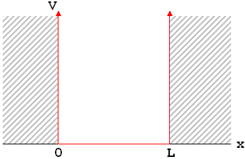
What this potential energy function tells you is that, within the range 0<x<L, the particle is free to move with no forces on it whatsoever. But at x=0 and x=L, there is an absolutely unstoppable force that pushes it back; so the particle just can't go there. For reasons that should hopefully be clear this example is often called a "particle in a box."
So, let's walk through the steps we outlined above. We will start by figuring out the energy eigenstates, using the time-independent Schrödinger equation.
![]()
On the left and right sides of the graph, V=![]() . Based on the equation (not based on the physical situation), what does that tell us about Y? Answer: if V=
. Based on the equation (not based on the physical situation), what does that tell us about Y? Answer: if V=![]() , there is only one way to prevent the middle term from blowing up, and that is to set Y=0. Of course, this mathematical result also tells us what we physically expect: the probability of the position being in this range is zero everywhere. The particle must be in the middle range.
, there is only one way to prevent the middle term from blowing up, and that is to set Y=0. Of course, this mathematical result also tells us what we physically expect: the probability of the position being in this range is zero everywhere. The particle must be in the middle range.
So, what about that range? There, where V=0, the above equation reduces to:
![]() =EYE
=EYE
This is one of the relatively few differential equations that you can solve just by looking at it right. You start by shoving all the constants over to the right side, for convenience.
![]()
In other words, the second derivative of YE gives you back minus YE, times a constant. It just so happens that both the sin and the cos fill that condition. And since it's a second order differential equation, we only need two linearly independent solutions for full generality, so we can write the answer immediately:
That solves the time-independent Schrödinger equation in the region 0<x<L. However, we still have to apply normalization and boundary conditions. The former we've discussed before and the latter comes about because the wavefunction has to be continuous. (If you like you can think of that as another postulate, but it's really required for the theory to work consistently.) Since we know Y=0 outside this range, we know it must approach 0 at x=0 and x=L. Plugging in Y(0)=0 immediately gives B=0, so one of our terms disappears right away! To get Y(L)=0 we could set A=0, but then we would have Y=0 everywhere, which is a non-physical solution because it can't be normalized. Thus the only way to satisfy our second boundary condition is to set the argument of the sine function to a multiple of p. In other words
![]()
What does that tell us? Remember that m and L are fixed parameters of the problem, so the only things that can vary in this equation are E and n. That means that this requirement fixes the possible values for E. Solving, we find that
![]()
where n can be any positive integer.
It's critical at this point to step back and say: what did we just discover? What we just discovered is that E is not free to be anything it wants to. There is a constant ![]() , which is big and ugly but still just a constant. For convenience we're going to call this constant E0 so we don't have to keep writing it out. E can be equal to E0, or it can be 4E0, or 9E0, or 16E0, but nothing in between. The energy is quantized: we didn't have to postulate that, the math just spit it out at us.
, which is big and ugly but still just a constant. For convenience we're going to call this constant E0 so we don't have to keep writing it out. E can be equal to E0, or it can be 4E0, or 9E0, or 16E0, but nothing in between. The energy is quantized: we didn't have to postulate that, the math just spit it out at us.
The final step in finding the energy eigenstates is to normalize this function to find the coefficient A. To do this we calculate
![]()
A couple of notes about this calculation: First, we take into account that in principle A could be complex. Second, we chose to rewrite E in terms of n because it's a little simpler, but we could have just left E in explicitly as well. To normalize YE we have to set this integral equal to one, so we get |A|2=2/L, which holds true for any A of the form A=eif![]() . The normalized energy eigenstates are thus
. The normalized energy eigenstates are thus
![]()
with corresponding energy eigenvalues given by E=E0n2
(We've left out the arbitrary phase in front of Yn.)
We're done with the hard part. Now, remember that at t=0, Y can be pretty much anything it wants (subject to the normalization and boundary conditions)—you can't figure out Y(0) from the potential energy, you have to be told Y(0) as an initial condition of the problem. So, just suppose someone tells you that at time t=0 the wavefunction for your particle is:
You can confirm that this is properly normalized. We're now going to ask and answer a number of questions about this wavefunction and the particle it describes. We strongly encourage you to try to answer them before looking at our answers.
Question 1: If you were to measure the energy of this particle at time t=0 what would you find?
Answer: The correct answer is that there is a 1/4 chance that you would find E=E0 and a 3/4 chance that you would find E=25E0. Note that after you did this measurement the wavefunction would change completely. Depending on what you got it would either become Y1 or Y5. In all the questions that follow we're going to assume you haven't done this or any other measurement before the one asked about in the question.
Question 2: If you were to measure the position of the particle at time t=0 what would you find?
Answer: The odds of your different results would be given, as always, by the probability distribution |Y|2. We've plotted this function below.

Question 3: What will the wavefunction be at some later time t?
Answer: Each energy eigenstate will be multiplied by a phase e-iE/![]() , so the wavefunction will be
, so the wavefunction will be
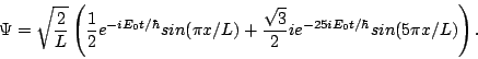
Question 4: If you measure the energy at time t what will you find?
Answer: Exactly the same thing you found at time t=0. Multiplying the coefficients by a phase doesn't change their magnitudes, so the odds of the two results are still 1/4 and 3/4.
Question 5: If you measure the position at time t what will you find?
Answer: Once again the probability distribution for position is given by |Y|2, but now that's a different function. Taking t=![]() /5E0, for example, the probability distribution will look like
/5E0, for example, the probability distribution will look like
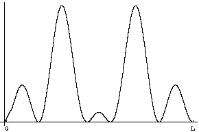
You should be able to check this yourself by plugging in t=![]() /5E0 into the equation above and calculating the squared magnitude. Phases do matter!
/5E0 into the equation above and calculating the squared magnitude. Phases do matter!
It all boils down to the following rules.
Purists may be annoyed by the fact that we have one general rule for finding every observable except position, and a completely different (albeit simpler) rule for position. Every other observable uses the operator to find the basis states, and work from there. Is there a basis state for position? The answer is, yes there is—you can treat position exactly the same way as any other observable, basis states and all. Click here if you want to see how.
We should note for the sake of completeness that not all observable quantities can be built out of position and momentum. For classical particles that's all there is, but quantum mechanical particles have an entirely new dynamic property called spin that's unrelated to position and momentum. The basic rules for spin are the same. There is a spin operator and there are spin basis states and so forth, but a full discussion of this would be beyond the scope of this paper.
Finally, we should note once more that once you have measured a quantity for a particular particle, that particle's wavefunction changes drastically. Whatever the probability distribution might have been for the quantity you are measuring, once you've measured it you know it has exactly the value you measured. For example, suppose a particle has the wavefunction
Y = 3/5 Y1 + 4/5 Y2
where Y1 and Y2 are eigenstates of some observable O with eigenvalues 2 and 7 respectively. The squared coefficients 9/25 and 16/25 tell you the probabilities that a measurement of O will give the results 2 or 7 respectively. If you make the measurement and find the result 2, however, then at that point the particle's wavefunction has become Y1. A subsequent measurement performed immediately afterwards is guaranteed to give you the result 2 again. This change that occurs in the wavefunction as a result of measurement is called the "collapse of the wavefunction," and it forms one of the principal differences between quantum and classical physics.
A real number is defined as one that has no i in it. An imaginary number is a real number times i (such as 4i). A complex number has both real and imaginary parts. Any complex number z can be written in the form x+iy where x and y are real numbers. x is the "real part" and y is the "imaginary part." For instance, 2+3i is a complex number.
The complex conjugate of a complex number, represented by a star next to the number, is the same real part but the negative imaginary part. So if z=2+3i then z*=2�3i. Note that the reverse is also true: if z=2�3i then z*=2+3i. So you always have two numbers that are complex conjugates of each other.
Real numbers can be graphed on a line (the number line). Complex numbers, since they have two separate components, are graphed on a plane called the "complex plane" where the real part is mapped to the x-axis, the imaginary part the y-axis. Every complex number exists at exactly one point on the complex plane: a few examples are given below.
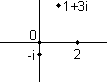
Every complex number has a magnitude which gives its distance from the origin (0) on the complex plane. So 1 and i both have magnitude 1. The magnitude is written with absolute value signs. So we can say that if z=2+3i then |z|2=22+32.
If you multiply any number by its own complex conjugate, you get the magnitude of the number squared (you should be able to convince yourself of this pretty easily). So we can write that, for any z, z*z=|z|2.
OK, but on average what number will you get? For instance, if you rolled the die a million times, and averaged all the results (divided the sum by a million), what would the answer probably be? This is called the "expectation value." You can probably see, intuitively, that the answer in this case is 2½. Never mind that an individual die roll can never come out 2½: on the average, we will land right in the middle of the 1-to-4 range, and that will be 2½.
But you can't guess the answer quite so easily if the odds are uneven. For instance, suppose the die is weighted so that we have a 1/2 chance of rolling a 1, a 1/4 chance of rolling a 2, a 1/8 chance of rolling a 3, and a 1/8 chance of rolling a 4? Your intuition should tell you that our average roll will now be a heck of a lot lower than 2½, since the lower numbers are much more likely. But exactly what will it be?
Well, let's roll a million dice, add them, and then divide by a million. How many 1s will we get? About 1/2 million. How many 2s? About 1/4 million. And we will get about 1/8 million each of 3s and 4s. So the total, when we add, will be (1/2 million)*1+(1/4 million)*2+(1/8 million)*3+(1/8 million)*4. And after we add—this is the kicker—we will divide the total by a million, so all those "millions" go away, and leave us with (1/2)1+(1/4)2+(1/8)3+(1/8)4=1 7/8.
The moral of the story is: to get the expectation value, you do a sum of each possible result multiplied by the probability of that result. This tells you what result you will find on average.
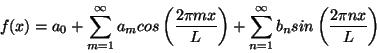
For each sine or cosine wave in this series the wavelength is given by L/m or L/n respectively. In other words the indices m and n indicate the wave number (one over wavelength) of each wave. Using the formula
eix=cos x + i sin x
you can rewrite the Fourier series in the equivalent form
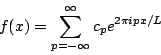
The function e2pipx/L is called a plane wave. Like a sine or cosine wave it has a value that oscillates periodically, only with plane waves this value is complex. That means that even if f(x) is a real function the coefficients cp will in general be complex. Either way you represent it, however, a Fourier series is simply a way of rewriting a periodic function f(x) as an infinite series of simple periodic functions with numerical coefficients.
A Fourier transform is the exact same thing, only f(x) doesn't have to be periodic. This means that the index p can now take on any real value instead of just integer values, and that the expansion is now an integral rather than a sum.
![]()
The factor of ![]() is a matter of convention and is set differently by different authors. Likewise some people add a factor (usually ±2p) in the exponential. The basic properties of the Fourier transform are unchanged by these differences. Note that this formula has nothing to do with position and momentum. The variable x could be position, or time, or anything else, and the variable p tells you the wave number (one over wavelength) of each plane wave in the expansion. (If x is time then the wave number is the same thing as the frequency of the wave.) To invert this formula, first multiply it by e—ip'x (where p' is just an arbitrary number) and then integrate with respect to x.
is a matter of convention and is set differently by different authors. Likewise some people add a factor (usually ±2p) in the exponential. The basic properties of the Fourier transform are unchanged by these differences. Note that this formula has nothing to do with position and momentum. The variable x could be position, or time, or anything else, and the variable p tells you the wave number (one over wavelength) of each plane wave in the expansion. (If x is time then the wave number is the same thing as the frequency of the wave.) To invert this formula, first multiply it by e—ip'x (where p' is just an arbitrary number) and then integrate with respect to x.
![]()
It is possible to evaluate the integrals on the right hand side of this equation, but doing so requires a familiarity with Dirac delta functions. If you are not familiar with these functions you can just skip the next paragraph and jump straight to the result. (We discuss Dirac delta functions in a later footnote, but if you're not already somewhat familiar with them trying to follow the argument below may be an exercise in frustration.)
The only x dependence in this integral comes in the exponential, which is an oscillatory function. If p-p' is anything other than zero then this exponential will have equal positive and negative contributions and the integral will come out to zero. (Actually eipx is complex so the equal contributions come from all directions in the complex plane. If you can't picture this just take our word for it.) If p-p' is zero, however, then the exponential is simply one everywhere and the x integral is infinite. Thus the x integral is a function of p-p' that is infinite at p-p', and zero everywhere else, which is to say a delta function. Of course this isn't a rigorous proof. It can be proven rigorously that the integral of a plane wave is a delta function, however, and when you do the math carefully you find that the integral produces a delta function with a coefficient of 2p. So
![]()
where the integration over p uses the defining characteristic of a delta function. Replacing the dummy variable name p' with p we finally arrive at the formula
![]()
We should emphasize once more that mathematically x is just the argument to the function f(x) and p is just the wave number of the plane waves in the expansion. The fact that the relationship between Y(x) and f(p) in quantum mechanics takes the form of a Fourier transform means that for a given wavefunction Y(x) the momentum happens to be inversely related to the wavelength. (Once again, though, a realistic wavefunction will be made of many waves with different wavelengths.)
We said before that the numerical coefficients in the Fourier transform definition were arbitrary. In quantum mechanics these coefficients pick up an extra factor of ![]() , so the full relation between Y(x) and f(p) is
, so the full relation between Y(x) and f(p) is
![]()
![]()
Finally, we should note one convenient theorem about Fourier transforms. Consider the normalization of the wavefunction, which is determined by the integral of its squared magnitude. Writing that in terms of the Fourier expansion we find
![]()
This result can be proven by taking the complex conjugate of the expression for Y(x) above, multiplying it by Y(x), and integrating over x using the same delta function trick we used above. We won't bother to show this proof here. Recall that f(p) is the coefficient of the momentum basis state with momentum p, so what this result says is that if the wavefunction is properly normalized so that the total probability of the position being anywhere is one, then it will automatically be normalized so that the total probability of the momentum having any value is one.
We can see how this comes out of the rules we've given so far by considering the basis states of momentum, which are of the form eipx/![]() , which is equal to cos(px/
, which is equal to cos(px/![]() )+i sin(px/
)+i sin(px/![]() ). In other words the basis states of momentum are waves whose wavelength is determined by the value p. (Specifically, the wavelength is 2p
). In other words the basis states of momentum are waves whose wavelength is determined by the value p. (Specifically, the wavelength is 2p![]() /p.) When you expand a wavefunction in momentum basis states you are writing Y(x) as a superposition of these waves.
/p.) When you expand a wavefunction in momentum basis states you are writing Y(x) as a superposition of these waves.
Those familiar with Fourier expansions know that a localized wave is made up of components with many different wavelengths. At the other extreme a function made up of a single wave isn't localized at all. If a particle is in a momentum eigenstates Y=eipx/![]() then its position probabilities are equally spread out over all space. The bigger the range of wavelengths contained in the superposition the more localized the function Y(x) can be. From this we can see that a particle highly localized in momentum (a small range of wavelengths for Y) will have a very uncertain position (Y(x) spread out over a large area), and a particle highly localized in position (Y(x) concentrated near a point) will have a very uncertain momentum (many wavelengths contributing to the Fourier Transform of Y). You can certainly cook up a wavefunction with a large uncertainty in both position and momentum, or one that's highly localized in one but uncertain in the other, but you can't make one that's highly localized in both.
then its position probabilities are equally spread out over all space. The bigger the range of wavelengths contained in the superposition the more localized the function Y(x) can be. From this we can see that a particle highly localized in momentum (a small range of wavelengths for Y) will have a very uncertain position (Y(x) spread out over a large area), and a particle highly localized in position (Y(x) concentrated near a point) will have a very uncertain momentum (many wavelengths contributing to the Fourier Transform of Y). You can certainly cook up a wavefunction with a large uncertainty in both position and momentum, or one that's highly localized in one but uncertain in the other, but you can't make one that's highly localized in both.
It's possible to make a mathematical definition of what you mean by the uncertainty in position or momentum and use the properties of Fourier Transforms to make this rule more precise. The rule ends up being that the product of the position uncertainty times the momentum uncertainty must always be at least ![]() /2.
/2.
OK, you say, but if it's that arbitrary, then why does it work? Why can we say that kinetic energy is p2/2m, so the kinetic energy operator will be found by squaring the momentum operator and then dividing by 2m? Well, to some extent, you have to accept the operators as postulates of the system. But it does make sense if you consider the special case of an operator corresponding to some observable acting on an eigenfunction. If Yp is an eigenfunction of momentum with eigenvalue p that means that a particle whose wavefunction is Yp must have a momentum of exactly p. In that case, though, its momentum squared must be exactly p2, which is the eigenvalue you get by acting on Yp with the momentum operator twice. So in the end, it's not quite as arbitrary as it first appears. (Of course, this is not a proof of anything, but hopefully it's a helpful hand-wave.)
![]()
where in the last step we've used the fact that the wavefunction must be normalized. For this special case we can see that our formula worked. What happens when Y is not an eigenfunction of O? For simplicity let's consider a wavefunction made up of just two basis states:
Y=C1Y1+C2Y2
We know for this case the correct answer for the expectation value of O is v1|C1|2+v2 |C2|2. To see how our formula gives us this result we act on Y with the operator O to get
OY=C1v1Y1+C2v2Y2
Our formula then tells us that
![]()
![]()
The first two terms look like exactly what we need since each basis state Yi is itself a valid wavefunction that must be properly normalized. (This is a bit more complicated for continuous variables, where the basis states are not normalized in this way, but a similar argument applies.) The last two terms seem to spoil the result, though. Here's the hand-waving part: for any two different basis states Y1 and Y2, the integral
![]()
will always be zero. The technical way to say this is that the basis states of all operators representing observables are orthogonal. This property, which we're not going to prove here, is the last necessary step to show why the expectation value formula works. (We do make an intuitive argument why this is true for the momentum basis states in our footnote on Fourier transforms.)
The best way to answer this is actually not mathematically, but physically. Remember that a basis function represents a state where the particle has exactly one value, and no probability of being any other value. But we know that you find probabilities of position by squaring the wavefunction. So if we want a function that says "the position must be exactly 5" then clearly this wavefunction must equal 0 at every point but x=5. But if the probability distribution is completely concentrated at one point then it must be infinitely high at that point!
This function—infinitely high at one point, zero everywhere else—is known as the Dirac delta function and is written as the Greek letter delta. So d(x-5) is the function that is infinitely high at x=5, and zero everywhere else, such that the total integral is 1. To make this definition mathematically rigorous, you have to define it as a limiting case of a function that gets thinner-and-taller while keeping its integral at 1.
We said earlier that the position operator is x (meaning "multiply by x"). Now we're saying that the delta function is the position basis function: in other words, the eigenfunction for that operator. So it should be true, for instance, that xY=5Y when Y=d(5). In one sense we can see that this is true. Since d(x-5)=0 everywhere except x=5 multiplying it by x can only have an effect at the point x=5. So we can say that xd(x-5)=5d(x-5). At the same time, it seems kind of silly to multiply an infinitely large number by 5. What it really means is that the integral of the delta function, which was 1 by definition, will now be equal to 5.
Of course the above explanation isn't at all rigorous mathematically. In fact the "definition" we gave of the Dirac delta function was pretty hand-waving. The more rigorous definition involves taking the limit of a series of functions that get thinner and taller around x=5 while keeping their total integral equal to 1. If you think about multiplying one of these tall, narrow functions by x and then integrating you should be able to convince yourself that you get the same narrow function, only five times taller.
x''(t)=-k/m x(t)
An equation like this is called an ordinary differential equation (ODE) because the dependent variable, namely the function x that you are solving for, depends only on one independent variable, t. You can write down a general solution to this equation, but it will necessarily have undetermined constants in it. Because this is a second order ODE it has two undetermined constants. The full solution of this particular equation is
x(t)=C1sin(![]() t)+C2cos(
t)+C2cos(![]() t)
t)
The undetermined constants C1 and C2 indicate that you can put any number there, and you will still have a solution: for instance, 2sin(![]() t)-¾cos(
t)-¾cos(![]() t) is one perfectly valid solution. To find the constants that should be used for a particular situation, you must specify two specific data, such as the initial conditions x(0) and x'(0). In other words if you know the state of your particle (position and velocity) at t=0 then you can solve for its state at any future time.
t) is one perfectly valid solution. To find the constants that should be used for a particular situation, you must specify two specific data, such as the initial conditions x(0) and x'(0). In other words if you know the state of your particle (position and velocity) at t=0 then you can solve for its state at any future time.
In quantum mechanics we have to deal with a partial differential equation (PDE), which is an equation where the dependent variable (Y in this case) depends on two independent variables (x and t). As a simple example of a PDE (simpler in some ways than Schrödinger's Equation) we can consider the wave equation
![]()
Here f(x,t) is some function of space and time (eg the height of a piece of string). Once again we can write down the general solution to this equation, but now instead of a couple of undetermined constants we have some entire undetermined functions!
f(x,t)=g1(x-t)+g2(x+t)
You can (and should) check for yourself that this solution works no matter what functions you put in for g1 and g2. You could write for example
f(x,t)=sin2(x-t)+ln(x+t)
and you would find that f satisfies the wave equation. How can you determine these functions? For the ODE above it was enough to specify two initial values, x(0) and x'(0). For this PDE we must specify two initial functions f(x,0) and f'(x,0) (where the prime here refers to a time derivative). For a piece of string, for instance, I must specify the height and velocity of each point on the string at time t=0, and then my solution to the wave equation can tell me the state of my system at any future time.
How does this apply to Schrödinger's Equation? Schrödinger's Equation is only first order in time derivatives, which means you can write the general solution in terms of only one undetermined function. In other words if I specify Y(x,0) that is enough to determine Y for all future times. (One way you can see this is by noting that if you know Y(x,0) Schrödinger's Equation tells you Y'(x,0), so it wouldn't be consistent to specify both of them separately.) So to solve for the evolution of a quantum system I must specify my initial wavefunction and then solve Schrödinger's Equation to see how it evolves in time.
 Gary and Kenny Felder's Math and Physics Help Home Page
www.felderbooks.com/papers
 Send comments or questions to the authors