Implementation Notes

CLUSTEREASY uses ``slab decomposition,'' meaning the grid is divided along a single dimension (the first spatial dimension). For example, in a 2D run with $N=8$ on two processors, each processor would cast a $4 \times 8$ grid for each field. At each processor the variable n stores the local size of the grid in the first dimension, so in this example each processor would store $n=4$, $N=8$. Note that n is not always the same for all processors, but it generally will be if the number of processors is a factor of N.

In practice, the grids are actually slightly larger than $n \times N$ because calculating spatial derivatives at a gridpoint requires knowing the neighboring values, so each processor actually has two additional columns for storing the values needed for these gradients. Continuing the example from the previous paragraph, each processor would store a $6 \times 8$ grid for each field. Within this grid the values $i=0$ and $i=5$ would be used for storing ``buffer'' values, and the actual evolution would be calculated in the range $1 \le i \le 4$, $0 \le j \le 7$.

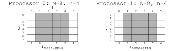
This scheme is shown above. At each time step each processor advances the field values in the shaded region, using the buffers to calculate spatial derivatives. Then the processors exchange edge data. At the bottom of the figure I've labeled the $i$ value of each column in the overall grid. During the exchange processor 0 would send the new values at $i_{totalgrid}=0$ and $i_{totalgrid}=3$ to processor 1, which would send the values at $i_{totalgrid}=4$ and $i_{totalgrid}=7$ to processor 0.

The actual arrays allocated by the program are even larger than this, however, because of the extra storage required by FFTW. When you Fourier Transform the fields the Nyquist modes are stored in extra positions in the last dimension, so the last dimension is $N+2$ instead of $N$. The total size per field of the array at each processor is thus typically $n+2$ in 1D, $(n+2) \times (N+2)$ in 2D and $(n+2) \times N \times (N+2)$ in 3D. In 2D FFTW sometimes requires extra storage for intermediate calculations as well, in which case the array may be somewhat larger than this, but usually not much. This does not occur in 3D.